7 Transformers from First Principles
Originally developed for machine translation, Transformers were introduced in the seminal 2017 paper Attention is All You Need (Vaswani et al. 2017). Since then, they have revolutionized the field of deep learning, and have become the de facto architectural basis for progress across a wide range of natural language processing tasks.
In the previous section, we discussed the parallels between DL models as a class, and ITTMs. Using this high-level understanding, we will now consider the Transformer architecture from first principles, using the tools of ITTMs and GDL to understand the model’s underlying behavior, structure, and limitations.
We will begin by examining the core building block of the Transformer model: the attention mechanism.
7.1 Attention and the Graph
The attention mechanism is the fundamental building block of the Transformer model. First conceptualized in 2014 (Bahdanau, Cho, and Bengio 2014), it allows the model to “focus” on different parts of the input sequence when generating the output sequence. This mechanism is inspired by the human ability to selectively focus on relevant information while ignoring irrelevant details.
Attention blocks are made up of two components, a process of multi-head self-attention and a multi-layer perceptron. The self-attention mechanism allows the model to weigh the importance of each input token when generating the output token. This process is repeated multiple times, with the output of each step being fed into its corresponding multi-layer perceptron.
This can be understood as a graph routing operation, where the model “queries” the input sequence to determine the importance of each token, and then “routes” this information to the output sequence. In this interpretation, the query operation occurs in the multi-head attention mechanism, while the routing operation is performed by the multi-layer perceptron. Each head corresponds to a different possible path, allowing the model to explore multiple possible future trajectories in a single step. Further, we know from the previous section that Transformer models approximate a fully-connected graph structure, making this routing operation over the graph particularly powerful.
7.2 Transformers as ITTM Implementations
In this section, we extend the correspondence between Deep Learning and ITTMs to the full architecture of the Transformer model. As established in Section 6.3.2, we can examine key processes of Transformer models and ITTMs using the framework of constituent components. These components outline the workflow that is common to both DL models and ITTMs, and allow us to draw parallels between the two.
Figure 7.2 illustrates the Transformer model as an ITTM, outlining the full input to output workflow, given sequences of symbolic data.
First, both models begin by processing input to discrete units processed by the respective model; in the case of the Transformer, data is resolved to tokens, while in the ITTM they are resolved to discrete states in the graph. Immediately following this, the input states are transformed to input-conditioned representations that correspond to underlying graph configurations. In Transformers, the output of this stage is an embedding; for ITTMs, the output is a node or set of nodes in the graph structure.
Following this, the Transformer model enters the hidden computation stage, where the input-conditioned graph representation is processed by the hidden attention blocks. These blocks are analogous to search and traversal operations over the nodes of the graph in the equivalent ITTM. Note that representations of different fully-connected computation graphs corresponding to possible model states at successive time steps beyond the first infinite successor ordinal (see Section 4.2), are stored in each of the hidden layer attention blocks in the Transformer model. Similarly, the ITTM stores sequences of computation graphs that are used to perform an equivalent computation.
Lastly, the final output of the hidden attention computation layers is converted back to a discrete unit in the decoder layer of the model. In the case of the ITTM, this corresponds to the output state of the model. Similarly, for a Transformer, this would be the output token from the computation of the model. Finally, the output token/state is mapped to the corresponding output symbol, completing the symbolic input to output sequence.
This alignment between Transformers and ITTMs simplifies the conceptual understanding of Transformer models by framing their operations as practical implementations of ITTM principles, such as graph-based computations and state transitions. With this isomorphism, each stage of a Transformer—from embedding tokens to traversing attention blocks and outputting symbols—can be understood as a structured traversal through a sequence of graph configurations, analogous to an ITTM progressing through transfinite computation steps. This perspective not only unifies the two paradigms but also enables a deeper analysis of Transformer performance characteristics from first principles, setting the stage for evaluating their scalability, efficiency, and fundamental computational constraints.
7.3 Paradox of Scale
Transformer models have shown remarkable performance across a wide range of tasks, from language modeling to motor control. In the domain of language modeling specifically, scaling up these models has led to impressive emergent behavior, such as the ability to generate coherent and contextually relevant text. This improvement in behavior by increasing the scale and scope of Transformer models has been used as justification for extremely large capital investments in infrastructure to drive increasing scale in the Transformer models.
However, as evidenced by the magnitude of these investments, scaling up Transformer models comes at a significant cost. The computational resources required to train and run these models are immense, with the largest models requiring thousands of Graphics Processing Units (GPUs) running in parallel for days, weeks, or even months to train.
In addition to the exorbitant costs associated with scaling up these models, there are diminishing returns on the performance improvements as the models scale. While increasing the size of the model and the amount of data used for training can lead to better performance, the rate of improvement decreases as the model grows larger. Furthermore, autoregressive models, which are commonly used in Transformer architectures, tend to suffer from accuracy drift as the model size increases. This diminishing return profile is a key factor in understanding the limits of scaling Transformer models.
This raises the question: why do these models require such vast resources to deliver results?
7.3.1 Neural Scaling Laws
The Neural Scaling Laws (Kaplan et al. 2020) provide a framework for understanding the relationship between model size, training data, and computational resources in deep learning models. While they were originally devised to analyze the performance of Transformers, subsequent research has shown that these scaling laws are applicable to a wide range of deep learning models.
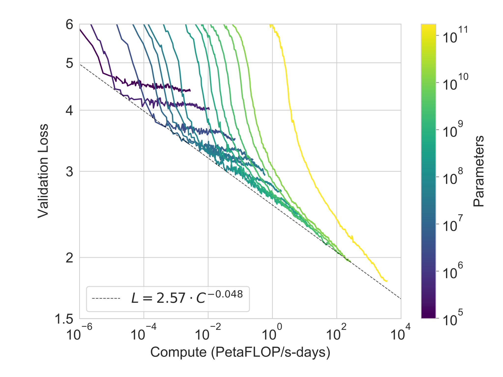
The laws describe how the performance of deep learning models scales with the number of parameters, the size of the training dataset, and the amount of compute used during training. The graphs show that there exists an efficient frontier in the scaling laws, beyond which increasing the size of the model, the amount of data, or the computational resources used does not lead to significant improvements in performance. This efficient frontier is govered by a power law, which describes the logarithmic relationship between model size, training data, and computational resources.
Analyzing this relationship through the lens of ITTMs, we can understand that the efficient frontier in the scaling laws corresponds to the maximum capacity of the underlying computation graph. The power law limit to scaling represents the saturation of the graph, where increasing the amount of data, or the computational resources used does not lead to significant improvements in performance, given a fixed model size.
As discussed in Section 6.3.1, the capacity of a Transformer model is set during the specification phase, when the hyperparameters of the model are defined. This capacity remains invariant to changes in the amount of data or computational resources used during training, leading to the logarithmic relationship observed in the scaling laws as the underlying graph approaches saturation.
Figure 7.3 depicts the efficient frontier for computational resources across different model sizes. More broadly, the scaling laws appear as a Pareto boundary along the compute and dataset axes. This boundary reflects the trade-off between the two resources: increasing either compute or dataset size beyond this point results in diminishing performance gains, constrained by the fixed model size and its corresponding computational graph capacity.
Through this analysis, we can see that the limits of scaling Transformer models are governed by a fundamental quantity; the capacity of the underlying computation graph, which is determined by the hyperparameters of the model. This framing provides a concrete theoretical basis for the diminishing returns observed in the performance of large Transformer models, and highlights a key limitation in the DL scaling paradigm.
7.3.2 Cost of Inference
Transformer models are inherently computationally expensive to run, requiring significant resources to perform inference on large datasets. This high cost of inference is due to the nature of the attention mechanism in the model, which involves routing over a fully-connected graph to determine the importance of each token in the input sequence. This routing operation is inherently an \(O(N^2)\) operation, where \(N\) is the number of tokens in the input sequence. Given that this operation is performed multiple times in each layer of the model, the overall complexity of inference in a Transformer model is \(O(L \times N^2)\), where \(L\) is the number of attention blocks in the model.
As discussed in Section 6.2, Transformer models encode fully-connected graph structures, where each token in the input sequence is connected to every other token. Notably, the routing operation over this fully-connected graph is inherently an \(O(N^2)\) operation, as it requires comparing each token to every other token in the sequence to determine the optimal path through the graph. Viewed through the lens of ITTMs, we can observe that this complexity arises from the fully-connected nature of the computation graph in the Transformer model, and is a fundamental property of the model architecture.
The \(O(N^2)\) complexity of inference in Transformer models has significant implications for the scalability of the model. As the size of the input sequence grows, the computational resources required to perform inference increase quadratically, making it increasingly expensive to run large Transformer models on long sequences. This trade-off between model size and computational cost is a key factor in understanding the limitations of Transformer models, the most performant of the DL architectures.
7.3.3 Autoregressive Accuracy Dropoff
Transformer models are commonly used in an autoregressive fashion to make predictions, where the model generates the output sequence token-by-token based on the input sequence. While this approach has been highly successful in a wide range of tasks, it is not without its limitations. One key challenge faced by autoregressive models, such as Transformers, is an exponential dropoff in accuracy as the length of the output sequence increases.
As outlined in Faith and Fate: Limits of Transformers on Compositionality (Dziri et al. 2023), the probability of a correct prediction, \(P_{\text{correct}}\), for a autoregressive model with probability \(\epsilon\) of making an error on each token decreases exponentially with the length of the output sequence, \(L\), according to the formula:
\[P_{\text{correct}} = (1 - \epsilon)^L\]
As illustrated in Figure 7.4, this exponential dropoff in accuracy stems from the nature of the depth-first traversal of the computation graph in autoregressive models. As the model generates each token in the output sequence sequentially, the probability of making an error on each token accumulates, leading to an exponential decrease in the overall accuracy of the model.
This can also be understood through the lens of a depth-first search over the ITTM graph, generalizing the concept to a broader class of DL models. Exponential accuracy dropoff is a fundamental limitation of autoregressive models, and significantly impacts the use of the Transformer architecture for long sequence generation tasks.
7.4 Improving the Transformer Architecture
Despite the limitations of the Transformer model, there have been significant advancements in the field of deep learning that have improved the performance of these models. In this section, we will discuss other DL architectures that are iterations of the transformer, and talk about how they will always be limited by the nature of the representation of the underlying ITTM computation graph. In no particular order, these architectures include:
State Space Models: State space models, such as Mamba (Gu and Dao 2023), enhance sequence modeling by discretizing the latent space and leveraging structured state dynamics to process sequences efficiently. This discretization allows models to manage long-range dependencies while maintaining scalability and reducing computational overhead. By enabling dynamic control over information propagation and forgetting, these models address limitations in traditional Transformer architectures, improving performance across diverse modalities like language, audio, and genomics. Through the lens of ITTMs, state space models enable improvements with a more efficient representation of the underlying computation graph, allowing for more performant routing and traversal operations.
Constrained Resolution Representations: Binary and ternary neural networks, such as BinaryConnect (Courbariaux, Bengio, and David 2015), constrain weights to discrete values (e.g., -1, 0, 1), effectively reducing computational complexity and memory usage. This discretization simplifies operations, replacing multiplications with additions, which enhances efficiency and scalability. Such models are particularly beneficial in scenarios where high precision is unnecessary, like certain language modeling and image classification tasks, offering a more resource-efficient alternative to traditional Transformer architectures. Binary models represent a departure from the continuous domain representation of the graph in traditional Transformer architectures, offering a more efficient and scalable alternative for representing the underlying ITTM computation graph.
Positional Embeddings: Recent advancements in positional embedding strategies, such as Relative Positional Encoding (RoPE) (Su et al. 2021), have improved the ability of models to capture positional information in the self-attention mechanism. By incorporating relative positional information into the embedding layer, these models enhance the model’s ability to attend to distant tokens in the input sequence, enabling more effective context modeling. Positional embedding strategies like RoPE allow for infinite context by routing many times over the same ITTM computation graphs, improving the model’s ability to capture complex relationships in sequences.
Mixture of Experts (MoE): MoE models (Shazeer et al. 2017) are an architecture that employs multiple specialized “expert” sub-models, dynamically selecting a subset of these experts for each input. This selective routing mechanism allows MoE models to scale to trillions of parameters while maintaining computational efficiency by activating only a small fraction of the model for any given task. While this segmentation enables greater capacity and efficiency, it comes with trade-offs, such as challenges in generalization and limited communication between experts. Under the ITTM interpretation, this has the effect of segmenting the computation graph into different experts, allowing for more efficient routing over the graph, but at the cost of reduced generalization.
Joint Embedding Predictive Architectures (JEPA): JEPA (LeCun 2022) represent a shift from traditional generative models towards a framework that directly learns predictive embeddings for structured data. Instead of reconstructing entire inputs, JEPA focuses on predicting latent representations, which significantly reduces computational complexity and allows for more efficient learning. This approach leverages a contrastive loss between embeddings of paired observations to model relationships within data, avoiding the need for explicit modeling of input distributions. This architecture can also be modeled as an ITTM, using a continuous domain representation of the graph, but with a different set of operators acting on the structure than Transformer models.
While these advancements have improved the performance and efficiency of deep learning models, they are still fundamentally limited by the core constraints of the continuous representation of the underlying computation graph. Furthermore, the high computational cost of inference, and diminishing returns on scaling inherent limitations of the Transformer architecture, and more broadly DL.
To overcome these limitations and achieve a more scalable, efficient, and generalizable architecture, we must look beyond the current DL paradigm and explore radically new approaches to building intelligent systems.