6 Deep Learning as an ITTM
In this section, we explore the conceptual alignment between Deep Learning (DL) and ITTMs, proposing a novel perspective on DL architectures as computational systems with the capacity to approximate ITTM processes. This section presents how DL models, especially when framed as geometric structures, can internalize complex relationships analogous to those managed by ITTMs, bridging theoretical ITTM operations and practical DL model operations.
By drawing on principles of Geometric Deep Learning (GDL), we reinterpret classical DL architectures as inherently graph-based, aligning their operations with the graph-theoretic frameworks that represent ITTMs. This reinterpretation not only illuminates the structural parallels between DL models and ITTMs but also emphasizes the role of deep learning in modeling and approximating transfinite computation-like processes. Through this lens, we aim to unify concepts from DL and ITTMs, setting the foundation for understanding how deep learning architectures are functional approximators of hypercomputational systems.
6.1 Geometric Deep Learning
Geometric Deep Learning (GDL) represents a unified framework to extend Deep Learning (DL) techniques to non-Euclidean data structures like graphs (Bronstein et al. 2021). It achieves this by formulating models as a sequence of operations that are designed to respect the geometric properties and invariances inherent in these structures. This shift enables a graph-centric view of DL, where neural networks are represented as graphs and operations are performed on these structures.
The core concept behind GDL is to deal with operations that preserve symmetries and invariances present in the data. These properties are crucial, as the ordering of nodes in a graph should not impact the outcomes of learning tasks. To achieve this, GDL employs permutation equivariant operations, which ensure that permuting the input does not alter the model’s interpretation of it.
By focusing on operations that preserve geometric properties like symmetry and invariance, GDL makes it possible to extend classical architectures, such as Convolutional Neural Networks (CNNs), Recurrent Neural Networks (RNNs), Long-Short Term Memory (LSTM) Networks, and Transformers, to a graph-centric representation. Using this principle, we use GDL to adapt familiar DL concepts like convolution, pooling, and attention to graph structures.
6.1.1 GDL Operators
GDL, as defined, relies on a set of core operators to effectively capture and model relationships in geometric data. The two primary categories of operators in GDL are permutation equivariant operators and pooling operators.
6.1.1.1 Permutation Equivariant Operators
Permutation equivariant operators ensure that a model’s output changes in a consistent manner when the input nodes are reordered. This is essential for graphs, where the ordering of nodes is arbitrary and should not impact the interpretation of relationships between them. For example, in models dealing with Transformer architectures, permutation equivariant operations allow each token or element to interact and exchange information with other tokens based solely on their underlying relationships, rather than their specific positions within the input sequence. This consistency is key to accurately capturing dependencies and relationships in tasks, where the emphasis is on the contextual connections rather than the specific order of tokens.
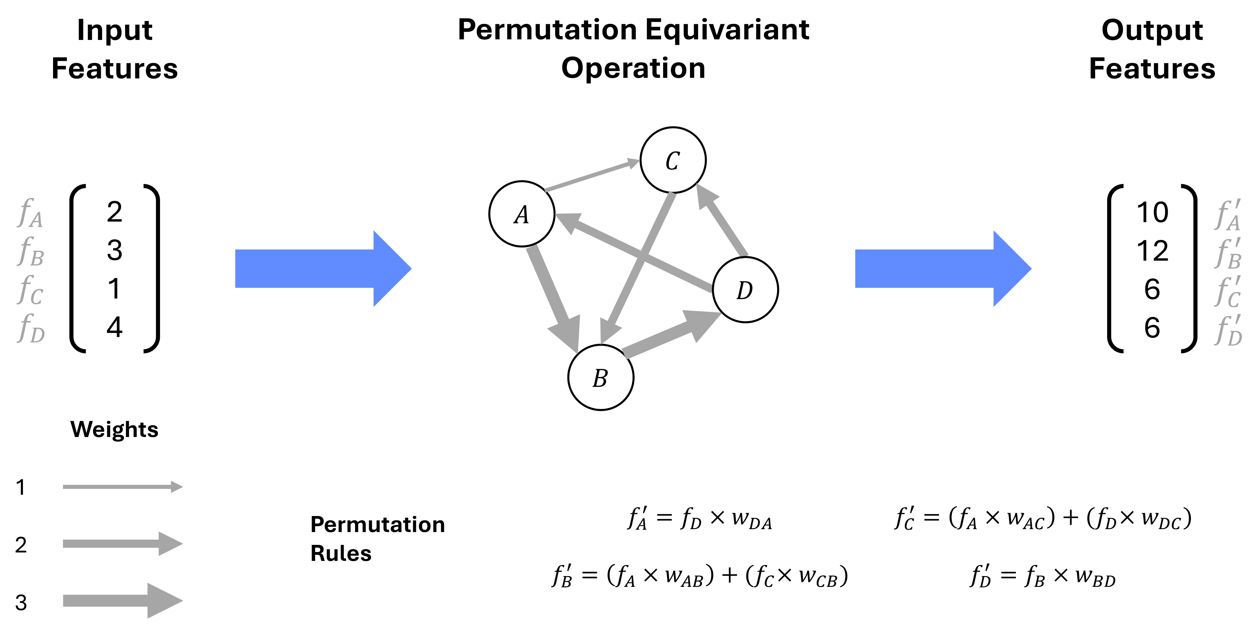
In the case of Figure 6.1, the permutation operation is conditioned on the underlying structure of the graph, and not the specific ordering of the nodes. This ensures that the model’s output remains consistent, as the premutation rules rely purely on the paths to the neighbors of each node, rather than an a priori ordering of nodes.
6.1.1.2 Pooling Operators
Pooling operators in GDL provide mechanisms to aggregate information from local neighborhoods or across entire structures. They are crucial for summarizing data at different scales, which is necessary for capturing both localized patterns and global characteristics of complex domains.
Local Pooling: Local pooling involves aggregating features from a node’s immediate neighborhood. This is analogous to the way traditional CNNs apply pooling operations over local patches of an image. In graph-based models, local pooling captures localized patterns and interactions by summarizing information from a node’s connected neighbors. For ITTMs, this allows the model to capture specific state transitions between closely related nodes.
Global Pooling: Global pooling aggregates information across an entire graph, providing a high-level summary of the structure. This operation is particularly useful when dealing with tasks that require understanding the overall behavior of a graph, such as graph classification or summarizing the state evolution of an ITTM. By condensing the entire graph’s information into a single representation, global pooling enables models to distill large-scale patterns that are relevant for capturing the comprehensive state of a model at specific points in its computation.
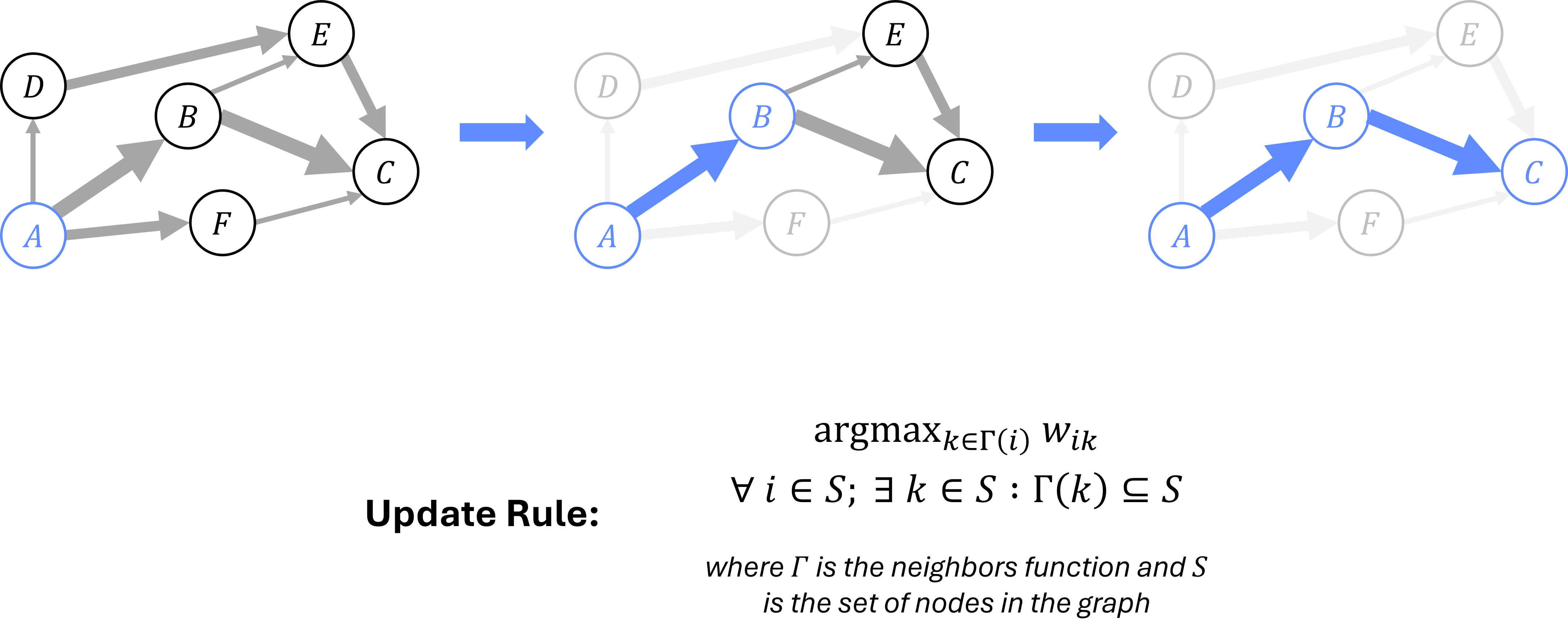
Figure 6.2 illustrates a local pooling operation, which summarizes information from a node’s immediate neighborhood; it can be used to select the most relevant path based on a specific rule. In this case, the routing operation selects the path with the highest weight at each node. Repeating this local pooling operation twice yields the complete route \(A\rightarrow B \rightarrow C\) when starting from node \(A\).
6.2 DL Models as Graph Structures
GDL was initially developed to extend traditional DL architectures—such as CNNs, RNNs, and Transformers—into non-Euclidean domains like graphs. This extension enabled models to handle irregular data structures while maintaining key invariances. However, in this paper, we adopt the inverse approach: instead of extending models to these spaces, we leverage GDL principles to reinterpret existing DL architectures as graph structures. By reversing the direction of this extension, we construct graph-based representations of classical neural network models and establish an isomorphism between these models and graphs.
This reinterpretation allows us to capture the relationships and dependencies within neural networks as connections and nodes in a graph, reflecting how information flows through layers and attention mechanisms. For instance, in a Transformer network, attention weights can be seen as dynamic edges between nodes, enabling the network to assign varying levels of importance to relationships between different elements. GDL formulates Transformer models specifically as a fully connected graph structure, where each node interacts with every other node, allowing for complex relationships to be captured.
By mapping these neural networks to graph representations using GDL principles, we create a consistent framework that justifies treating them as geometric objects, bridging the gap between theoretical models like ITTMs and modern DL architectures. This reverse perspective underpins our exploration of DL models as approximations of complex, graph-based theoretical systems.
This reinterpretation allows us to treat DL models as a specific representation of ITTMs with graph structures. By viewing DL models through the lens of Geometric DL, we can explore how these models internalize and manipulate complex relationships within state graphs, ultimately bridging the gap between theoretical computations and practical neural network operations. In the following sections, we will leverage existing vocabulary for the various processes and components that compose modern DL, and unify them with those of the ITTM. We will then use this understanding to discuss some of the limits of DL in the context of ITTMs.
6.3 Unifying DL and ITTM Concepts
Having established a basis for analyzing DL models as ITTMs, we can now establish relationships between key concepts in each domain. We survey key concepts in DL across two primary axes; DL lifecycle concepts and model components.
6.3.1 Deep Learning Lifecycle
DL models undergo a lifecycle that encompasses 3 main stages: training dataset and model construction, model training, and model inference. During the training dataset construction phase, the model’s training data is assembled, and model hyperparameters (specifying the model dimensions, layer count, etc.) are set. The training phase involves first randomly initializing the model weights and setting algorithm hyperparameters, then tuning those model weights over the set of training data using backpropagation (Rumelhart, Hinton, and Williams 1986) to guide parameter optimization. Finally, the model inference phase involves using the trained model to make predictions or perform other tasks.
| Phase | DL Term | ITTM Term | Description |
|---|---|---|---|
| 1 | Construction | Specification | Assemble training data, specify machine parameters (if any), etc. |
| 2 | Training | Compilation | Accelerate the machine through infinity and calibrate transfinite time step representations. |
| 3 | Inference | Execution | Utilize the representations to perform computations. |
We identify the lifecycle concepts for the ITTM alongside their corresponding DL terms in Table 6.1. While the specifics differ, the overall structure of the lifecycle remains consistent across both domains. This alignment allows us to draw parallels between the training and execution of DL models and the compilation and execution of theoretical ITTMs.
A key distinction in DL models is that the size of the model - and thus the size of the resulting ITTM graph representation - is specified at construction (phase 1), before the model has been exposed to any training data (phase 2). This pre-defined size represents a hard limit on the information capacity of the underlying graph, regardless of other variables. Further, due to the mechanics of these models, this size cannot be changed once phase 2 has begun, limiting the flexibility of DL approaches.
Stated differently, with DL architectures, we start by pre-defining a limit on the size of the computational model artifact, before exposing the artifact to the data over which it willl be performing computations. This inherently imposes an upper bound on the possible performance of a given DL system, as the model’s capacity to learn is fundamentally constrained by the initial size of the model.
6.3.2 Model Components
Building on the lifecycle concepts, we can explore the components that make up DL models and their relationships with ITTMs. The fundamental components of DL models can be broadly categorized into the following stages:
Input Data: The input data that the model processes, which can be tokens (in language models), image patches (in vision models), sequential states (in time-series models), or other arbitrary forms of information.
Input Transformation: This stage involves transforming the raw input data into a representation suitable for further computation. For instance, in NLP models, encoder layers may convert sequences of tokens into embeddings.
Core Computation: The model’s core architecture performs its operations. This could involve layers like LSTMs, self-attention, convolutional layers, or fully connected layers. Operations in this stage correspond to operations on the graph structure.
Output Transformation: After the core computation stage, the model transforms the intermediate results to generate the final output. This could involve additional layers, activation functions, or other transformations.
Output Data: Finally, the model outputs the processed data, which could be tokens, labels, images, or other forms of information, depending on the task.
Figure 6.3 illustrates a canonical DL model, as well as a theoretical ITTM, using the component categories outlined above. As implied, we interpret the core computation stages of various DL architectures (LSTM, CNN, RNN, etc.) as corresponding to operations performed on the graph structure of an ITTM. We assert there exists an isomorphism between various modern DL architectures and the graph structures of ITTMs.
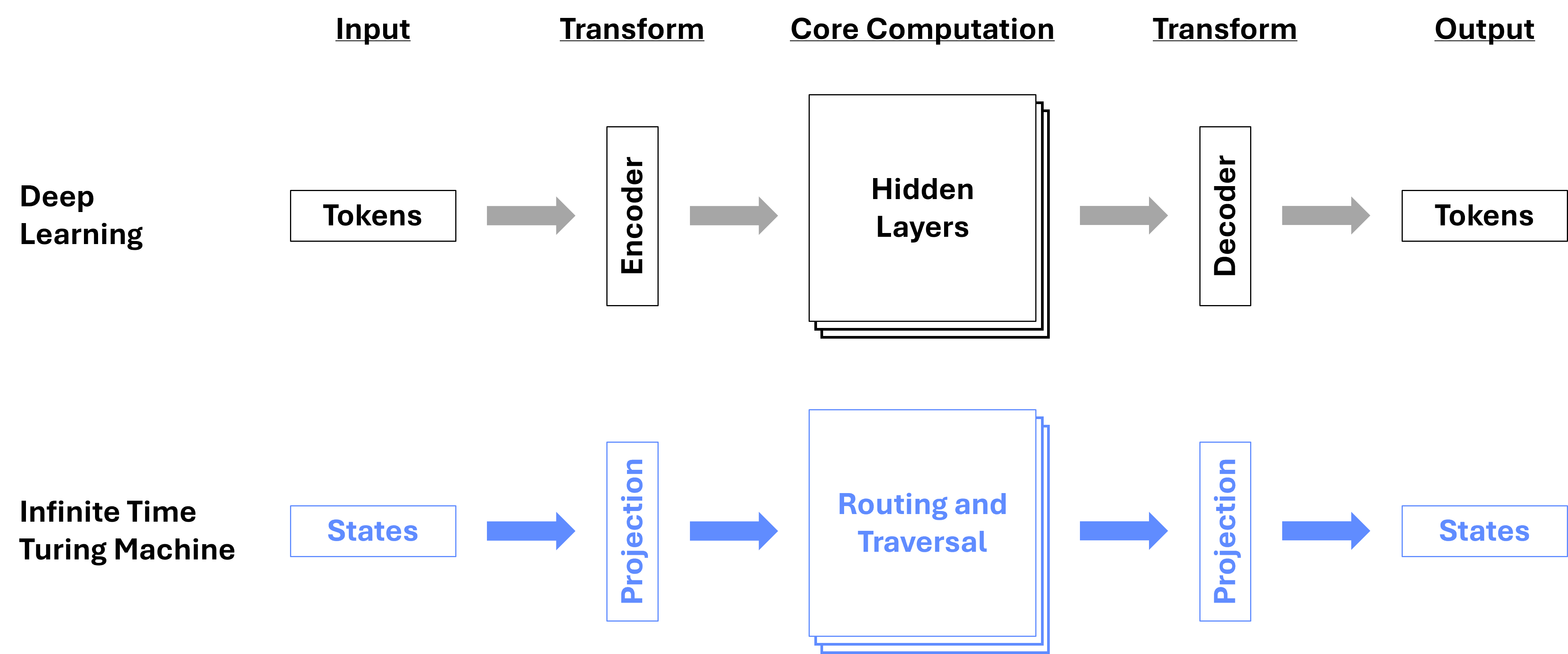
Expanding on this isomorphism, we can establish a direct correspondence between the components of DL models and the operations of ITTMs. For instance, we can consider the set of possible embeddings in a DL model as corresponding to the set of graph configurations in an ITTM. The transitions between states in an ITTM are akin to the operations in a DL model, where the operations in the DL model correspond to routing and traversal in an ITTM graph. Similarly, we can make connections between the encoder and decoder components of DL and the process of identifying specific configuration states in an ITTM during projection; the encoding process translates tokens to the graph domain representation, and the decoding process performs the inverse operation.
Further, we can extend this correspondence to the various architectures that enable different routing and traversal behaviors and enables the representation of graphs of arbitrary structure. By establishing this isomorphism, we can draw parallels between the components of DL models and the operations of ITTMs, providing a unified framework for understanding the relationships between these two domains.