3 Representations of Turing Machines

Turing Machines can be represented in various ways, each emphasizing different aspects of their behavior and structure. These representations are essential for understanding the mechanics of computation and the theoretical foundation behind algorithms. As we explore different representations of Turing Machines, we will set the stage for later discussions on how these concepts extend to more advanced models, like the ITTM.

The most common and rigorous way to represent a Turing Machine is through a formal mathematical description, typically defined as a 7-tuple. This formalism encapsulates the complete structure of the machine, including its states, symbols, and the rules that govern its behavior.

3.1 Formal Representations of Turing Machines

A Turing Machine can be formally represented as a 7-tuple: \[ M=(Q,\Sigma,\Gamma,\delta,q_0,q_{accept},q_{reject}) \]

Each element of this tuple describes a specific aspect of the machine:

\(Q\): A finite set of states. This defines all possible conditions the machine can be in during computation.
\(\Sigma\): The input alphabet, excluding the blank symbol B. This is the set of symbols that can appear on the tape as part of the input.
\(\Gamma\): The tape alphabet, which includes all symbols the machine can use during computation, including the blank symbol B. This alphabet typically includes the input alphabet and may have additional symbols for internal processing.
\(\delta\): The transition function. This function governs how the machine moves from one state to another based on the current state and the symbol being read. Formally, \(\delta : Q \times \Gamma \rightarrow Q \times \Gamma \times \{L,R\}\), where \(L\) and \(R\) represent the movement of the tape head (left or right).
\(q_0\): The initial state. This is the state the machine starts in when computation begins.
\(q_{accept}\): The accept state. If the machine enters this state, it halts and accepts the input.
\(q_{reject}\): The reject state. If the machine enters this state, it halts and rejects the input.

3.2 Transition Rules as a Graph

Another powerful way to represent the behavior of a Turing Machine is through transition graphs. In this form, the states and transition rules of the machine are visualized as a directed graph, where nodes represent the states and edges represent transitions between these states based on the input symbols. Each edge is labeled with the symbol being read, the symbol to write, the direction to move, and the next state to transition to.

We depict the transition rules of the binary counter machine from the previous section in the form of a graph:

Each state (such as \(q_0\), \(q_1\), and \(q_h\)) is represented as a node.
Edges between these nodes show the transitions between states, labeled with the input symbol, the output symbol, and the direction (left or right) that the read/write head moves.

Figure 3.1: Transition rules for the Binary Counter Turing Machine can be expressed as a graph.

In Figure 3.1, for the binary counter Turing Machine:

An edge from \(q_0\) to \(q_1\) indicates that when the machine reads 1, it writes 0, moves left, and transitions to state \(q_1\) (the carry state).
Another edge from \(q_1\) to \(q_h\) indicates that if it reads B (blank), it writes 1, moves right, and transitions to the halting state.

The graph-based representation provides a clear, visual understanding of how a Turing Machine works, illustrating an alternative inpterpretation for their behavior.

3.3 Machine Configurations as Composite States

To fully capture the dynamic behavior of a Turing Machine, we can represent the machine’s entire configuration at any given moment as a composite state. This approach goes beyond the simple transition graph by incorporating not only the machine’s current state but also the exact position of the read/write head on the tape and the current contents of the tape.

These composite states, or machine configurations, provide a more granular view of the machine’s status during computation. Instead of just knowing which state the machine is in (e.g., \(q_0\), \(q_1\), or \(q_h\)), a machine configuration includes:

The current state of the machine.
The current rule being applied (based on the current state and tape symbol).
The current tape contents.
The position of the read/write head on the tape.

This method of representation allows us to define distinct states that are far more specific than the high-level states represented in the transition graph. Each of these configurations can be indexed as \(s_t\), where \(t\) represents a unique snapshot of the machine at a particular time step \(t\).

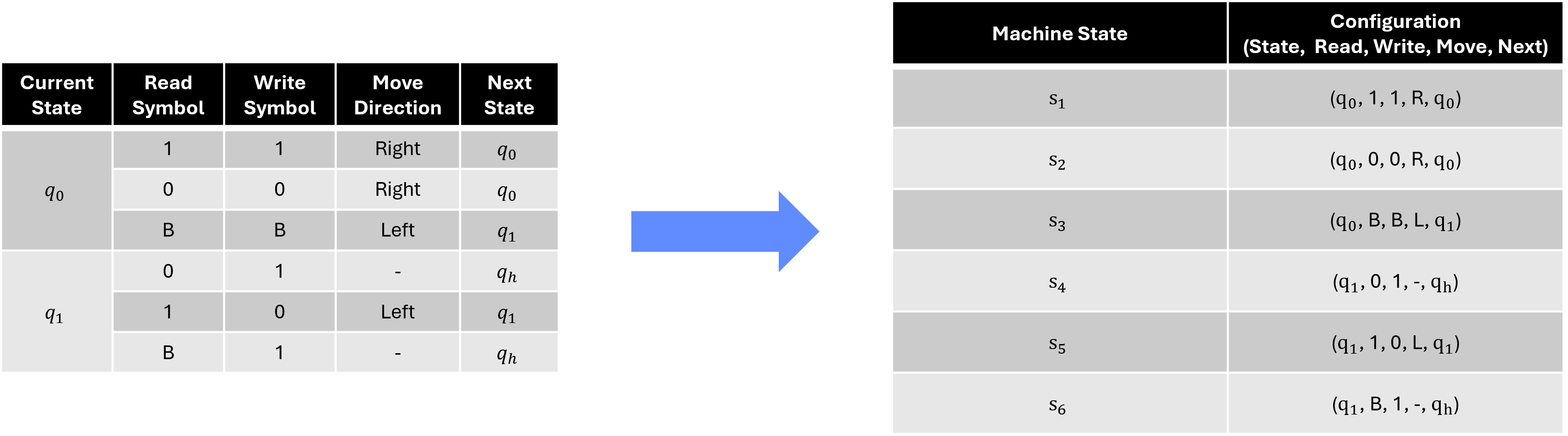
Figure 3.2: Machine configurations of the Binary Counter Turing Machine.

Figure 3.2 depicts these composite states for the binary counter example:

The machine transitions from one configuration to the next based on the current tape symbol, the state, and the movement of the head.
Each discrete machine state \(s_t\) is a snapshot of the entire machine at a particular step in the computation, representing the exact position of the read/write head and the tape contents at the corresponding position.

By considering the machine states as configurations that combine both state and tape information, we create a much richer model that shows the complete evolution of the machine through each computation step. This is especially useful when analyzing more complex behaviors, particularly cases where the movement of the head and modifications to the tape can only be opaquely inferred from the high-level state transitions.

This expanded representation complements the compressed transition graph by making it possible to track every computational step in detail, rather than just focusing on high-level state transitions. It provides a clear picture of how the machine evolves over time, allowing for a more thorough analysis of the computation process.

3.4 Machine Evolution Through Time

Building on the previous sections, where we explored representing a Turing Machine’s transition rules as a graph and capturing machine states, we can now look at how these representations evolve over time. Specifically, we can visualize the machine’s operation as a sequence of composite machine configurations, indexed by each time step. These configurations represent a complete snapshot of the machine at a given moment, including its state, the contents of the tape, and the position of the read/write head.

At each time step, the machine transitions to a new configuration based on the current state and tape symbol. This sequence shows how the machine’s composite state changes over time as it processes input, moving step-by-step through its transitions. In this representation:

Each composite configuration includes the current state, the entire tape (or relevant portion), and the position of the read/write head.
The sequence of configurations over time captures the evolution of the machine as it processes input, performing operations and transitioning through arbitrary states.

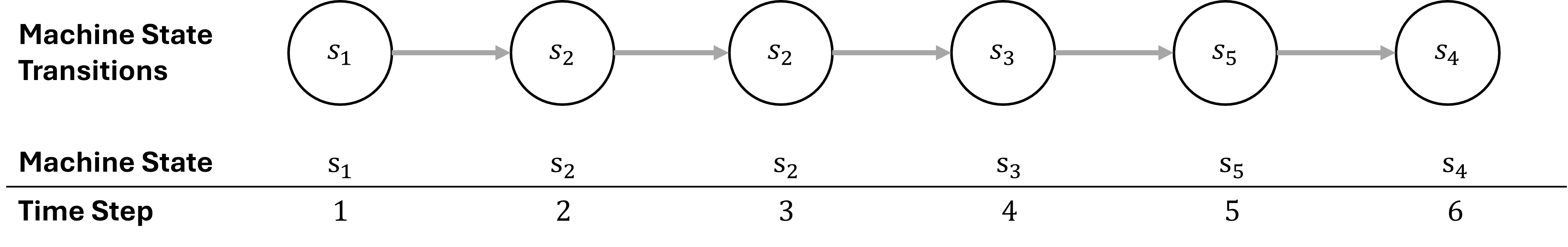
Figure 3.3: Expressing the evolution of a Turing Machine through time as a graph, combining the concepts of machine configurations as states with a graphical representation of the transition rules.

For example, for an arbitrary machine \(M\), we can represent each stage of the computation as a series of composite states, showing how the machine gradually approaches the correct output. Taking inspiration from Section 3.2, we can visualize the machine’s evolution not just as a series of snapshots, but also as a graph, with each transition representing a distinct configuration at a specific time step of the machine, resulting in a sequential graph of machine state transitions.