5 Representing Infinite Time Turing Machines
The goal of this section is to extend current research and present an abstract framework for representing ITTMs, focusing on how these machines evolve and operate over infinite and transfinite time steps. We introduce a series of graph-based representations to capture the behavior of ITTMs, including collapsed machine state graphs, probabilistic graphs that accommodate multiple computations, and sequential graphs representing the machine’s states at different transfinite ordinal steps.
These representations help us distill complex state transitions into manageable structures, enabling analysis and insights into the machine’s computations. Finally, we explore how these state graphs can be expressed as matrices or tensors, establishing connections to mathematical tools and deep learning architectures. Together, these representations provide a comprehensive foundation for understanding ITTMs and their capabilities across infinite sequences of time.
5.1 Collapsed Machine State Graphs
When analyzing the behavior of Turing machines, especially those operating over infinite time scales, it becomes impractical to consider every individual state transition. We can collapse the machine’s temporal sequence of states into a more compact form known as a collapsed machine state graph.
To do this, we need to understand how to represent a Turing Machine as it evolves over ordinal time steps, as it computes the result for a single program. We can then treat this resulting representation as a collapsed “point in time” representation of the machine as it processes the given program.
One strategy for this is to collapse repeated states into a single node, and encode the “path” of computation through time in the edges. This allows us to create a more compact representation of the machine’s behavior, focusing on the unique configurations encountered during the computation. Furthermore, it provides a high-level, temporally collapsed view of the computation, implicitly identifying patterns like cycles, convergence, or termination.
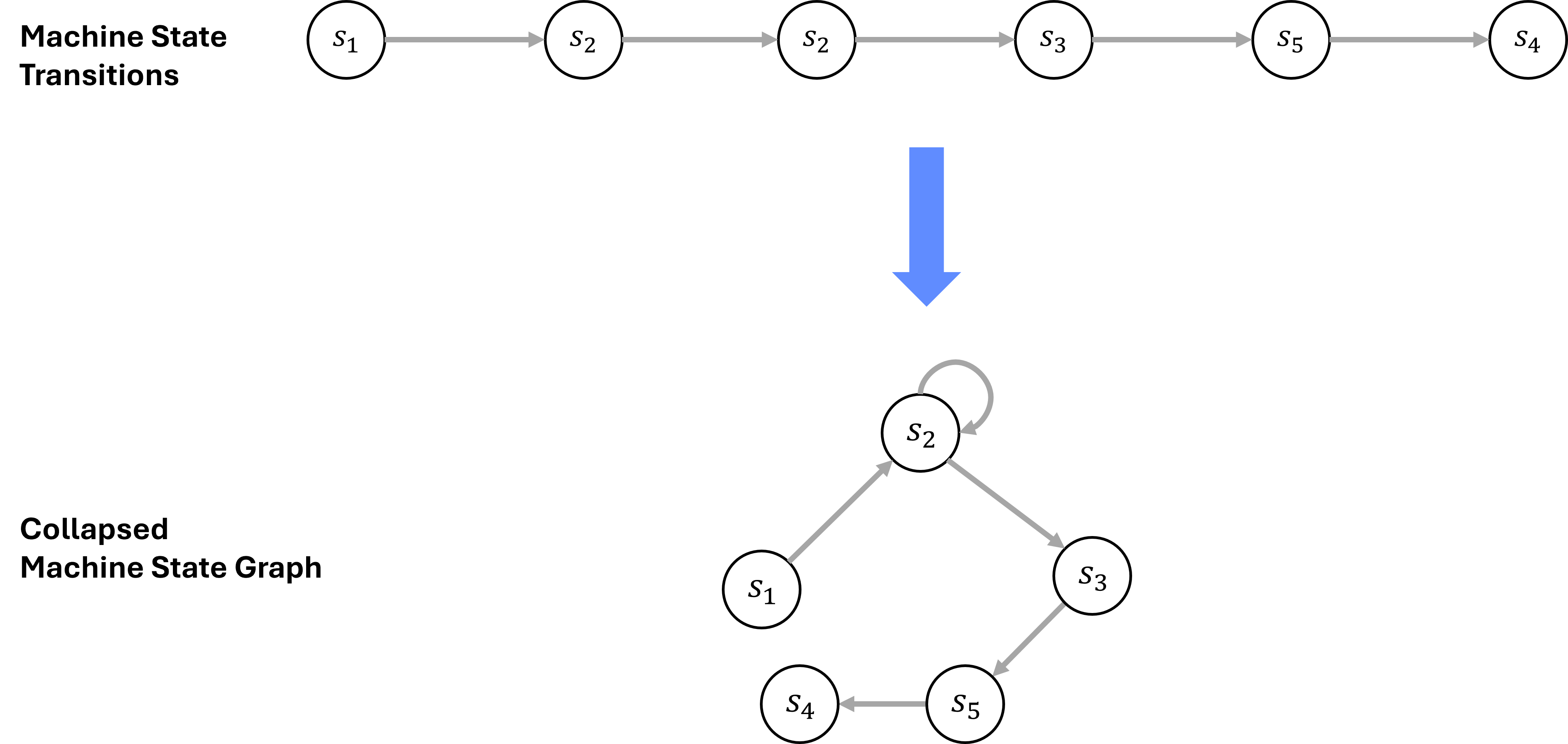
Figure 5.1 returns to the binary counter example and the notion of representing machine states over time from Section 3.4. We collapse the repeated state, \(s_2\), to a single node, representing the repetition with an additional edge. This simplifies the graph structure while preserving the essential structure of the state evolution. This collapsed machine state graph provides a temporally compressed view of the machine’s computation, while preserving each discrete transition in the computation.
5.2 Probabilistic Machine State Graphs
As we consider multiple programs or inputs processed by a Turing machine, we encounter a variety of possible state transitions and paths through the machine’s configuration space. To capture this variety, we extend the collapsed machine state graph into a probabilistic machine state graph. This graph captures the distribution of possible states and transitions that arise from processing different programs over time, in a single temporally-collapsed representation.
We achieve this by combining the collapsed machine state graphs for multiple independent program executions, and utilizing the edge distributions to create a probabilistic representation of the machine’s behavior. This allows us to derive a probabilistic representation out of exclusively computations, by keeping track of the transitions between machine configuration states during the computation.
This probabilistic machine state graph provides a powerful tool for modeling the behavior of machines across multiple programs computations, or computations over multiple inputs. It allows us to represent the cumulative effect of different programs on the machine’s state evolution. This means that we have derived a probabilistic system out of deterministic computations, which is a powerful concept in the context of ITTMs.
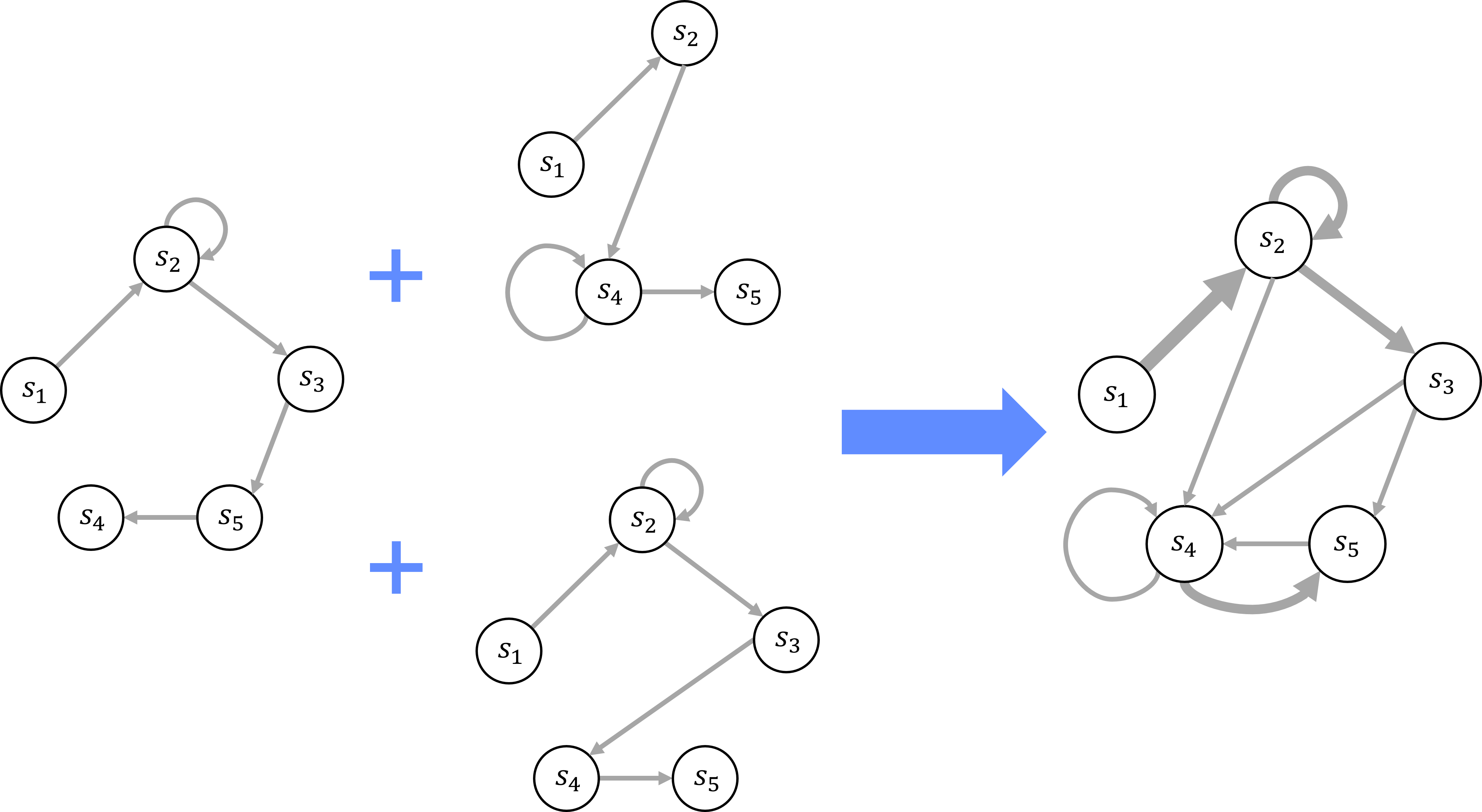
Figure 5.2 illustrates the composition of multiple collapsed machine state graphs into a single probabilistic machine state graph. Each edge in the graph represents a transition between machine configuration states during a program computation, with varying weights proportional to the likelihood of that transition occurring. By combining the edge distributions from different program computations, we create a probabilistic representation of the machine’s behavior computing multiple programs, over time. This representation temporally compresses and captures the cumulative effect of processing multiple programs into a single graph, and provides a basis to derive a probabilistic representation of the machine’s behavior from entirely deterministic computations.
Similar to the collapsed machine state graph, the probabilistic machine state graph represents a point-in-time structure that captures the possible states and transitions of the machine at a specific time step. By combining the edge distributions from multiple program computations, we create a comprehensive representation of the machine’s behavior over time, distilled into a single graph, temporally condensing the representation. This represents the machine’s evolution across multiple programs or inputs, capturing all possible states and transitions that that the machine could have undergone at a given point in transfinite ordinal time.
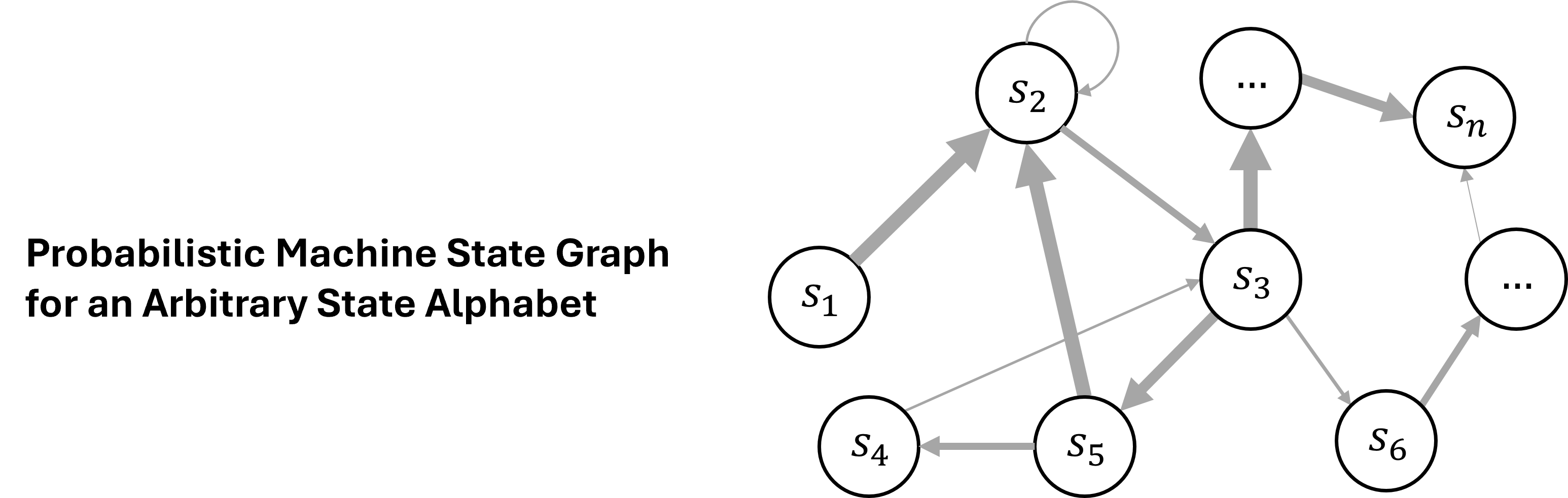
This notion extends naturally to arbitrary state alphabets, which we refer to as symbols. By representing each symbol in the alphabet as a node or set of nodes within the graph, we can theoretically accommodate machines with large or even infinite sets of states or symbols. This approach allows us to capture the expected evolution of the machine at a temporally collapsed point in time for any arbitrary state alphabet. This generalization is crucial when dealing with ITTMs, which may operate over infinite tapes (and correspondingly, have an infinite set of machine configuration states). Thus, we can model machines with arbitrary machine configuration state alphabets, \(s_1, \dots, s_n\), and represent their behavior over time using the probabilistic machine state graph representation approach as illustrated in Figure 5.3. Note that this arbitrary state alphabet can also be thought of as analogous to the symbols of the ITTM.
5.3 Representing Machines at Transfinite Time Steps
ITTMs extend the concept of computation beyond finite time steps into transfinite ordinal time steps such as \(\omega\), \(\omega + 1\), and so forth. To represent the state of an ITTM at these infinite points, we utilize the probabilistic machine state graphs developed earlier.
At the transfinite time step \(\omega\), the machine has completed an infinite sequence of computations. The machine’s state at this point, often referred to as the “limit state,” emerges from the cumulative sequence of configurations up to \(\omega\). We represent this limit state using a collapsed probabilistic graph, which encapsulates the machine’s composite behavior after this infinite sequence of computations. This allows us to create a snapshot of the machine’s state at \(\omega\), preserving the essential transitions while simplifying the representation.
For successor ordinals \(\omega + 1\), \(\omega + 2\), and beyond, we construct sequential representations to capture the state transitions at each of these infinite steps. These successive graphs build upon each other, reflecting the continued evolution of the ITTM into higher transfinite time points. Each representation encodes the cumulative effects of preceding configurations, providing a structured and hierarchical view of the machine’s behavior.
This hierarchical representation mirrors the layers of a deep learning model, where each layer processes the output of the previous one. Similarly, the ITTM’s state at each transfinite time step depends on its state at earlier steps, allowing us to model complex computations that unfold over infinite transfinite ordinal time steps.
As illustrated in Figure 5.4, we can represent the state of the ITTM at arbitrary transfinite ordinal time steps using sequences of probabilistic machine state graphs. Each graph captures the possible states and transitions of the machine at a specific point in transfinite ordinal time, providing a snapshot of the machine’s behavior at that time step. Note that the connections between states in each graph can vary significantly, reflecting the machine’s possible evolution over different transfinite ordinal time steps. Arbitrary sequences of these probabilistic machine state graphs allow us to represent ITTM configurations at arbitrary transfinite ordinal time steps.
5.3.1 Computations as Traversals
In this framework, computations in ITTMs are not merely represented as traversals through the state graphs; rather, the traversals are a natural consequence of the computations themselves. Each edge in the state graph reflects a specific transition executed by the ITTM, capturing the progression from one state to another as the machine processes its input.
To perform a computation within this framework, we effectively replay the corresponding sequence of transitions encoded within the graph. This means that following a path through the state graph is analogous to executing the original computation that generated the graph. Thus, the computation is embodied by the traversal, where each node and edge encapsulates a unique machine configuration and transition that occurred during the process.
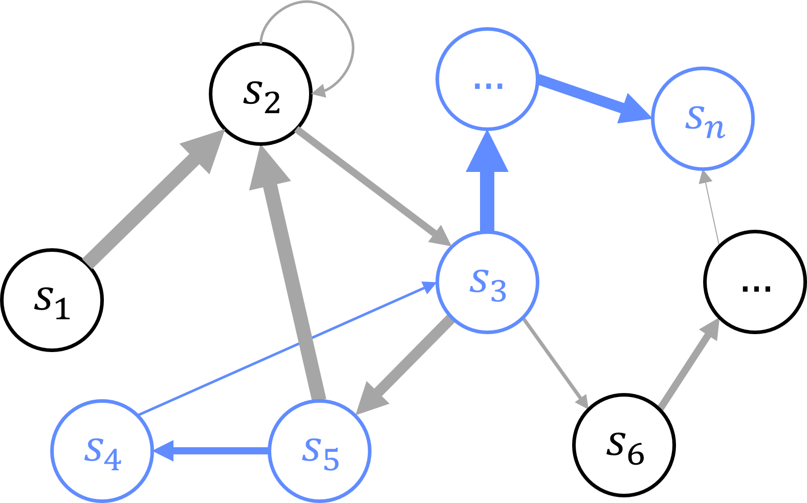
The notion of “routing” through these graphs ties directly into understanding the computation, as illustrated in Figure 5.5. When an ITTM encounters a specific input or set of instructions, the corresponding graph provides a blueprint for the sequence of states the machine will navigate. This traversal process can therefore be seen as the act of computation itself, allowing us to traverse paths through the graph to achieve specific outcomes.
Note that in the case of ITTMs operating over multiple transfinite ordinal time steps, this traversal process would occur over successive probabilistic machine state graphs, reflecting the machine’s evolution at each transfinite ordinal time step. By navigating these graphs, we effectively model the computations that the ITTM would perform at that transfinite time step.
5.4 Matrix and Tensor Encodings of Graphs
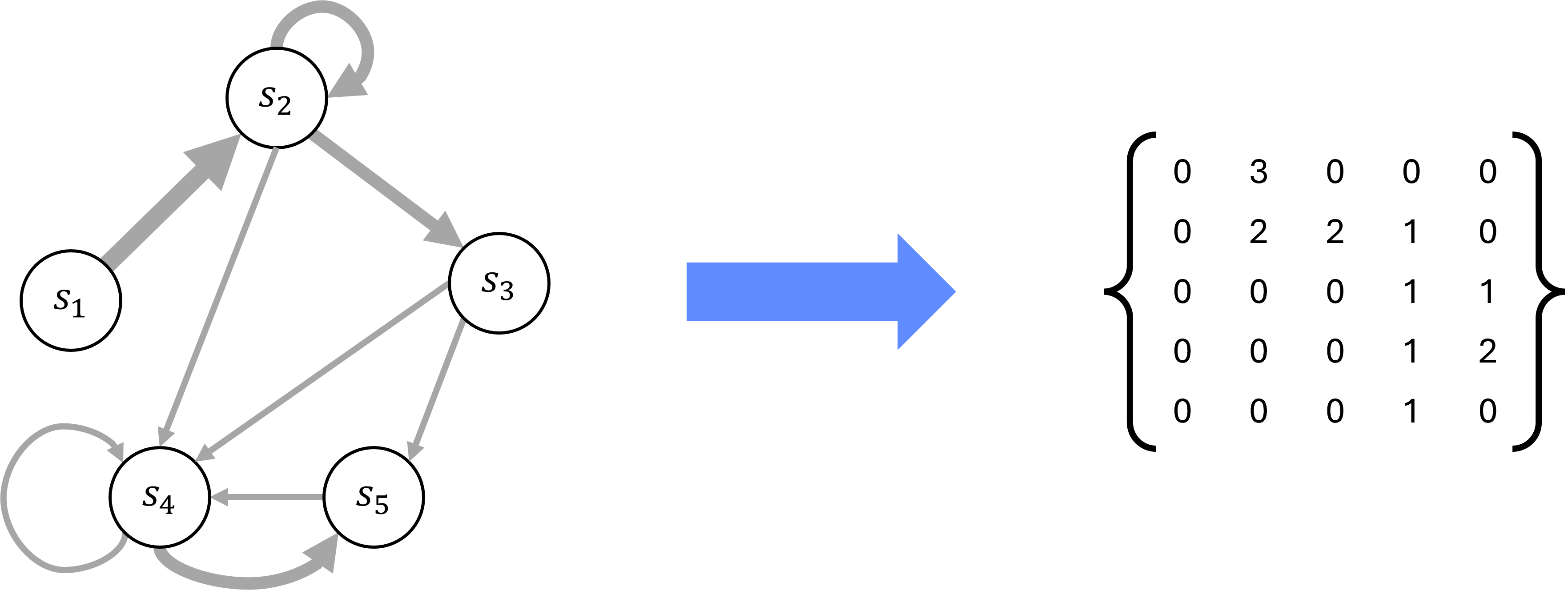
When representing complex systems like ITTMs, expressing their state graphs as matrices or higher-dimensional tensors becomes a powerful tool for analysis. Each graph, which captures state transitions and their probabilities, can be directly encoded into a matrix where the rows and columns correspond to the machine’s states. The entries in this matrix reflect the likelihood or frequency of transitions between pairs of states. This matrix-based approach not only provides a compact representation of the graph but also opens up opportunities to apply linear algebraic methods to study the machine’s behavior.
Figure 5.6 depicts an encoding of a graph as a 2-dimensional matrix. More generally, graphs can be encoded as \(n\)-dimensional tensors, where \(n\) denotes the dimensionality of the data being captured. For instance, a matrix is a 2-dimensional tensor capturing relationships between pairs of states, but more complex relationships or interactions (such as those involving three or more states) could be represented using 3-dimensional or higher-order tensors. This flexibility in dimensionality allows us to abstractly represent state graphs in a form that can capture multi-level dependencies and interactions within the graph.
In the context of deep learning, this representation is particularly significant. The hidden layers of neural networks often learn to capture, project, and encode complex relationships in the input data. If we consider state graphs as representations of sequential relationships or transitions within a computational system, it follows that hidden layers can effectively encode these graphs in matrix or tensor form.
As we will explore further in the next section, this suggests a parallel between the learned representations in deep learning networks and the structured encodings of state transitions in ITTMs. By expressing graphs as matrices or tensors, we bridge a conceptual gap between traditional graph representations and neural network architectures, laying the groundwork for understanding how deep learning models internalize and manipulate structured information.